MuMax3-How-To

Installation, scripting, & data generation demo of computational micro and nanomagnetism in MuMax3. Formed & written by Onri Jay Benally.

---

---

Main MuMax3 website: (https://mumax.github.io/index.html)

Uses code heavily-modified for clarity, inspired from: (https://github.com/mumax/3) & (https://mumax.github.io/examples.html)

Some examples computed in this repository were performed on an Nvidia (RTX 4070 Ti Super) GPU, connected externally (via a Thunderbolt 4 to PCIe x16 adapter) to a Microsoft Surface Pro 8, later upgraded to a Surface Pro 10. If you are curious about this kind of GPU-accelerated computing setup, then it is best to make sure your Windows machine is Thunderbolt 4 compatible or greater. Other examples were computed directly in the Google Colab environment using available GPU resources in Colab (T4 [free], L40, A100, etc.)

---

To use MuMax3 in Google Colab, simply change the runtime type to one of the GPU accelerators and enter this into the first code cell:

#@title Check GPU + driver
!nvidia-smi --query-gpu="name,driver_version,compute_cap" --format=csv

Then, enter this into the second code cell:

#@title Install MuMax³ (MuMax³ 3.10 CUDA 10.1)
# Download the mumax3 binary
!wget -q https://mumax.ugent.be/mumax3-binaries/mumax3.10_linux_cuda10.1.tar.gz
!tar -xvf mumax3.10_linux_cuda10.1.tar.gz
!rm mumax3.10_linux_cuda10.1.tar.gz
!rm -rf mumax3.10 && mv mumax3.10_linux_cuda10.1 mumax3.10

# Update the PATH environment variable
import os
os.environ["PATH"] += ":/content/mumax3.10"

Now you can write the MuMax3 code and Python visualization scripts in the remaining cells. See the Google Colab notebook examples for more information.

---

Here are some Colab Notebook examples you can try yourself:

https://github.com/OJB-Quantum/MuMax3-How-To/tree/main/Python%20Code_MuMax3%20Data%20Plots

--

Some Google Colab Notebooks
Run MuMax3 on the Cloud
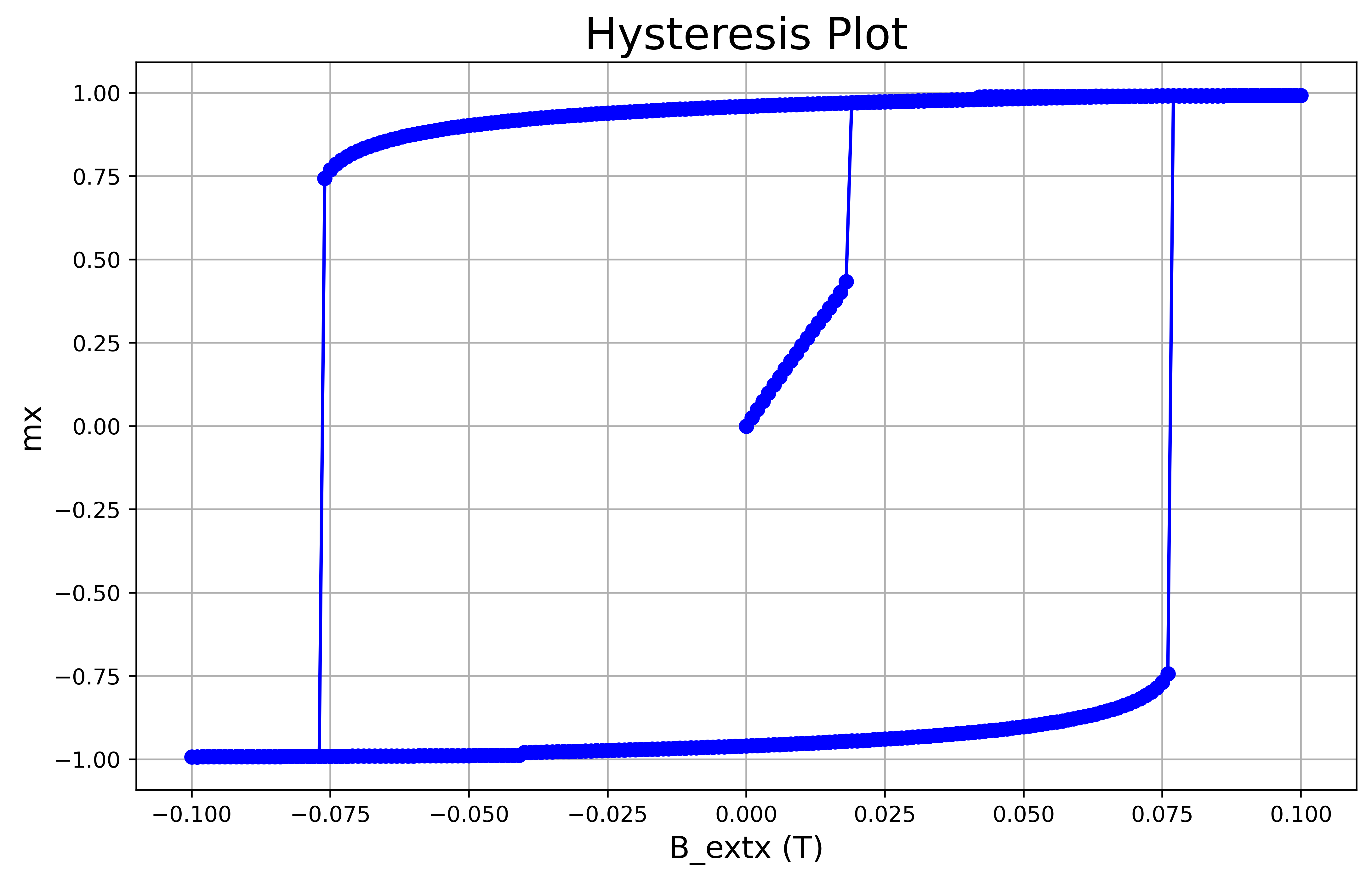
Example of Hysteresis Loop Data Imported from a Local MuMax3 Installation
Hysteresis Loop for Dy and Tb Micromagnets
Prediction of Temperature Dependence for Dy and Tb
Domain Wall Motion on Permalloy
STT Switching Simulation on MgO CFB pMTJ
Magnon Propagation Simulation
YIG & CFB Magnonics Simulation

---

How to Install & Run MuMax3 Locally by Onri
Video Tutorial on How to Install MuMax3 Locally Step-by-Step
The Official MuMax3 Tutorials
Standard Problems from the Center for Theoretical and Computational Materials Science (CTCMS)
Video Example of Onri's MuMax3 Hysteresis Plots in Python
Example MuMax3 Script in TXT Format
Video Animation of Magnetic Orders
Explanation of Hysteresis Curves & Coercivity
Micromagnetism Overview

---

If MuMax3 is installed already, start the GUI by typing the following 2 lines into a non-admin command prompt or non-admin PowerShell:

cd <directory_to_your_MuMax3_file>

mumax3 -i <your_MuMax3_TXT_file_name.txt>

Note: MuMax3 scripts can be written as TXT file types. The above script will load and automatically run the script into a browser.

Online OVF file type visualization: (https://mumax.ugent.be/mumax-view). While using the viewer, you can load multiple OVF files to play an animation of the magnetization frame capture.

---

Magnetic Unit Comparison Table

Quantity	Symbol	CGS Unit	SI Unit
Field	$H$	$\mathrm{Oe}$	$\mathrm{A\cdot m^{-1}}$
Flux	$\Phi$	$\mathrm{Mx}$	$\mathrm{Wb}$
Flux density	$B$	$\mathrm{G}$	$\mathrm{T}$
Magnetic moment	$m$	$\mathrm{emu}$	$\mathrm{A\cdot m^{2}}$
Magnetization per unit volume	$M$	$\mathrm{emu\cdot cm^{-3}}$	$\mathrm{A\cdot m^{-1}}$
Volume saturation magnetization	$M_{\mathrm{s}}$	$\mathrm{emu\cdot cm^{-3}}$	$\mathrm{A\cdot m^{-1}}$
Magnetization per unit mass	$\sigma$	$\mathrm{emu\cdot g^{-1}}$	$\mathrm{A\cdot m^{2}\cdot kg^{-1}}$
Mass saturation magnetization	$\sigma_{\mathrm{s}}$	$\mathrm{emu\cdot g^{-1}}$	$\mathrm{A\cdot m^{2}\cdot kg^{-1}}$
Magnetic polarization	$J$	$\mathrm{emu\cdot cm^{-3}}$	$\mathrm{T}$
Saturation magnetic polarization	$J_{\mathrm{s}}$	$\mathrm{emu\cdot cm^{-3}}$	$\mathrm{T}$
Volume susceptibility	$\chi_{\mathrm{v}}$	$\mathrm{emu\cdot Oe^{-1}\cdot cm^{-3}}$	dimensionless
Mass susceptibility	$\chi_{\mathrm{m}}$	$\mathrm{cm^{3}\cdot g^{-1}}$	$\mathrm{m^{3}\cdot kg^{-1}}$
Permeability	$\mu$	$\mathrm{G\cdot Oe^{-1}}$	$\mathrm{T\cdot m\cdot A^{-1}}$
Relative permeability	$\mu_{\mathrm{r}}$	dimensionless	dimensionless
Energy density	$W$	$\mathrm{erg\cdot cm^{-3}}$	$\mathrm{J\cdot m^{-3}}$
Demagnetizing factor	$N$	dimensionless	dimensionless
Energy product	$(BH)$	$\mathrm{MG\cdot Oe}$	$\mathrm{kJ\cdot m^{-3}}$

Mx = maxwell, G = gauss, Oe = oersted, Wb = weber, T = tesla, m = meter, A = ampere, J = joule, kg = kilogram, g = gram, cm = centimeter, emu = electromagnetic unit.

Magnetic Conversion Table

Quantity	Symbol	Conversion
Field	$H$	$\dfrac{\mathrm{Oe}}{\mathrm{A}\cdot\mathrm{m}^{-1}}=\dfrac{10^{3}}{4\pi}=79.6$
Flux	$\Phi$	$\dfrac{\mathrm{Mx}}{\mathrm{Wb}}=\dfrac{\mathrm{Mx}}{\mathrm{V}\cdot\mathrm{s}}=10^{-8}$
Flux density	$B$	$\dfrac{\mathrm{G}}{\mathrm{T}}=\dfrac{\mathrm{G}}{\mathrm{Wb}\cdot\mathrm{m}^{-2}}=10^{-4}$
Magnetic moment	$m$	$\dfrac{\mathrm{emu}}{\mathrm{A}\cdot\mathrm{m}^{2}}=\dfrac{\mathrm{erg}\cdot\mathrm{Oe}^{-1}}{\mathrm{A}\cdot\mathrm{m}^{2}}=\dfrac{10,\mathrm{A}\cdot\mathrm{cm}^{2}}{\mathrm{A}\cdot\mathrm{m}^{2}}=\dfrac{\mathrm{emu}}{\mathrm{J}\cdot\mathrm{T}^{-1}}=10^{-3}$
Magnetization per unit volume	$M$	$\dfrac{\mathrm{emu}\cdot\mathrm{cm}^{-3}}{\mathrm{A}\cdot\mathrm{m}^{-1}}=\dfrac{\left(\mathrm{erg}\cdot\mathrm{Oe}^{-1}\right)\cdot\mathrm{cm}^{-3}}{\mathrm{A}\cdot\mathrm{m}^{-1}}=10^{3}$
Volume saturation magnetization	$M_{\mathrm{s}}$	$\dfrac{\mathrm{emu}\cdot\mathrm{cm}^{-3}}{\mathrm{A}\cdot\mathrm{m}^{-1}}=\dfrac{\left(\mathrm{erg}\cdot\mathrm{Oe}^{-1}\right)\cdot\mathrm{cm}^{-3}}{\mathrm{A}\cdot\mathrm{m}^{-1}}=10^{3}$
Magnetization per unit mass	$\sigma$	$\dfrac{\mathrm{emu}\cdot\mathrm{g}^{-1}}{\left(\mathrm{A}\cdot\mathrm{m}^{2}\right)\cdot\mathrm{kg}^{-1}}=\dfrac{\left(\mathrm{erg}\cdot\mathrm{Oe}^{-1}\right)\cdot\mathrm{g}^{-1}}{\left(\mathrm{A}\cdot\mathrm{m}^{2}\right)\cdot\mathrm{kg}^{-1}}=1$
Mass saturation magnetization	$\sigma_{\mathrm{s}}$	$\dfrac{\mathrm{emu}\cdot\mathrm{g}^{-1}}{\left(\mathrm{A}\cdot\mathrm{m}^{2}\right)\cdot\mathrm{kg}^{-1}}=\dfrac{\left(\mathrm{erg}\cdot\mathrm{Oe}^{-1}\right)\cdot\mathrm{g}^{-1}}{\left(\mathrm{A}\cdot\mathrm{m}^{2}\right)\cdot\mathrm{kg}^{-1}}=1$
Magnetic polarization	$J$	$\dfrac{\mathrm{emu}\cdot\mathrm{cm}^{-3}}{\mathrm{T}}=\dfrac{\left(\mathrm{erg}\cdot\mathrm{Oe}^{-1}\right)\cdot\mathrm{cm}^{-3}}{\mathrm{T}}=10^{3}\mu_{0}=4\pi\cdot10^{-4}$
Saturation magnetic polarization	$J_{\mathrm{s}}$	$\dfrac{\mathrm{emu}\cdot{cm}^{-3}}{\mathrm{T}}=\dfrac{\left(\mathrm{erg}\cdot\mathrm{Oe}^{-1}\right)\cdot\mathrm{cm}^{-3}}{\mathrm{T}}=10^{3}\mu_{0}=4\pi\cdot10^{-4}$
Volume susceptibility	$\chi_{\mathrm{v}}$	$\dfrac{\left(\mathrm{emu}\cdot\mathrm{Oe}^{-1}\right)\cdot\mathrm{cm}^{-3}}{\left(\mathrm{A}\cdot\mathrm{m}^{2}\right)\cdot\left(\mathrm{A}\cdot\mathrm{m}^{-1}\right)^{-1}\cdot\mathrm{m}^{-3}}=4\pi$
Mass susceptibility	$\chi_{\mathrm{m}}$	$\dfrac{\left(\mathrm{emu}\cdot\mathrm{Oe}^{-1}\right)\cdot\mathrm{g}^{-1}}{\left(\mathrm{A}\cdot{m}^{2}\right)\cdot\left(\mathrm{A}\cdot\mathrm{m}^{-1}\right)^{-1}\cdot\mathrm{kg}^{-1}}=4\pi\cdot10^{-3}$
Permeability	$\mu=\dfrac{B}{H}$	$\dfrac{\mathrm{G}\cdot\mathrm{Oe}^{-1}}{\mathrm{T}\cdot\left(\mathrm{A}\cdot\mathrm{m}^{-1}\right)^{-1}}=\mu_{0}=4\pi\cdot10^{-7}$
Relative permeability (SI)	$\mu_{\mathrm{r}}$	$\dfrac{\mu_{\mathrm{SI}}}{\mu_{0}}=\mu_{\mathrm{r}}=\mu_{\mathrm{cgs}}$
Energy density	$W$	$\dfrac{\mathrm{erg}\cdot\mathrm{cm}^{-3}}{\mathrm{J}\cdot\mathrm{m}^{-3}}=0.1$
Demagnetizing factor	$N$	$\dfrac{N_{\mathrm{cgs}}}{N_{\mathrm{SI}}}=4\pi$
Energy product	$(BH)$	$\dfrac{\mathrm{G}\cdot\mathrm{Oe}}{\mathrm{T}\cdot\left(\mathrm{A}\cdot\mathrm{m}^{-1}\right)}=\dfrac{\mathrm{G}\cdot\mathrm{Oe}}{\mathrm{J}\cdot\mathrm{m}^{-3}}=4\pi\cdot10^{1}=126$ $\dfrac{\mathrm{MG}\cdot\mathrm{Oe}}{\mathrm{kJ}\cdot\mathrm{m}^{-3}}=4\pi\cdot10^{-2}=0.126$

Mx = maxwell, G = gauss, Oe = oersted, Wb = weber, V = volt, s = second, T = tesla, m = meter, A = ampere, J = joule, kg = kilogram, g = gram, cm = centimeter, with $\mu_0=4\pi\times10^{-7}$.

---

Hysteresis loop, from the local MuMax3 computation data:

---

Hysteresis loops for dysprosium at various low temperatures, from the MuMax3 Colab computation:

---

Magnetic material visualization example ran in MuMax3:

---

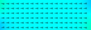
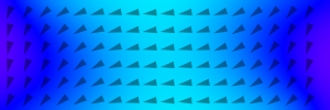
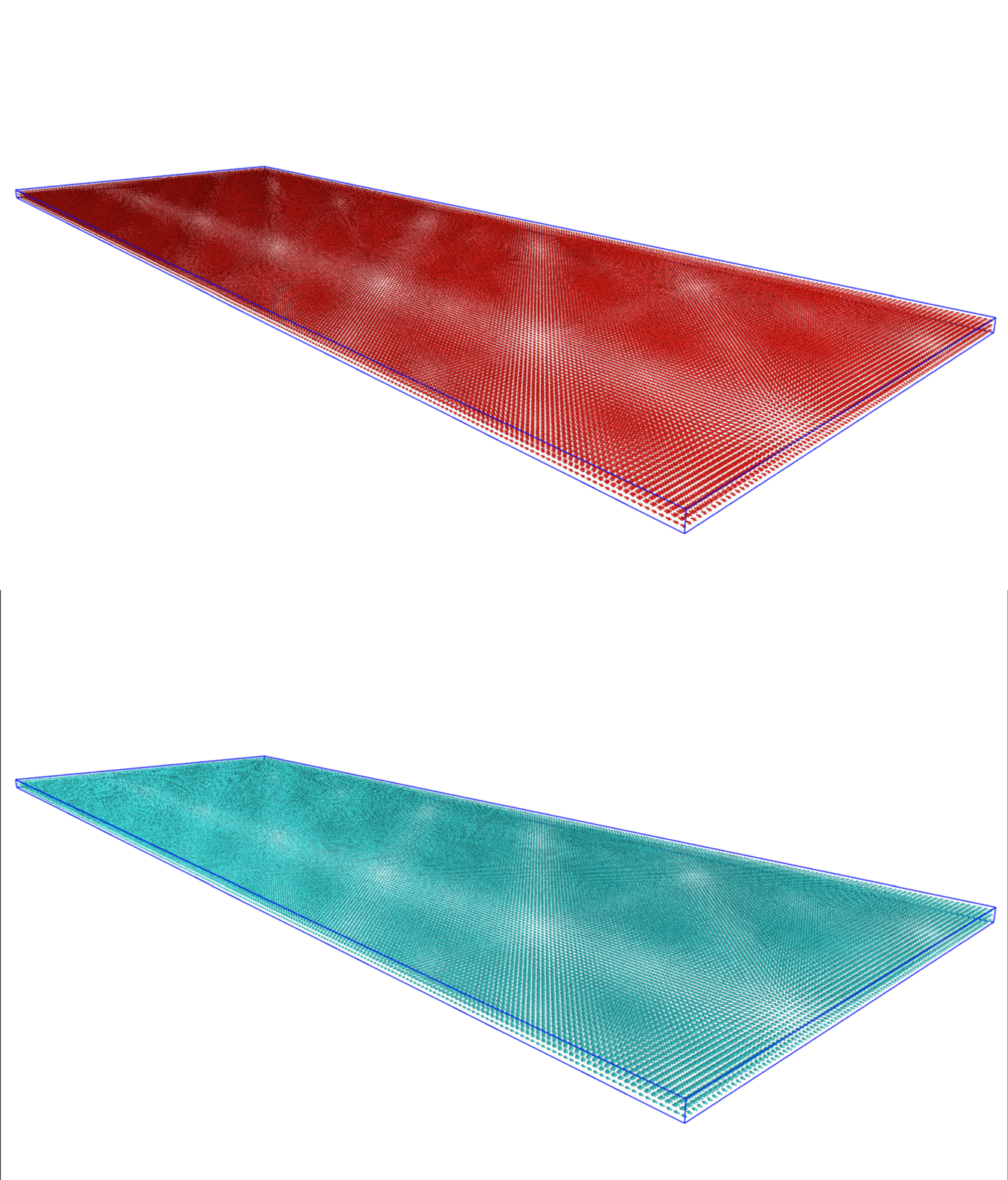
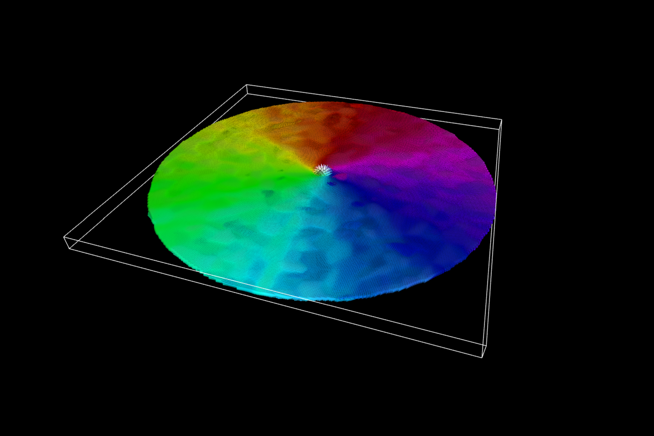
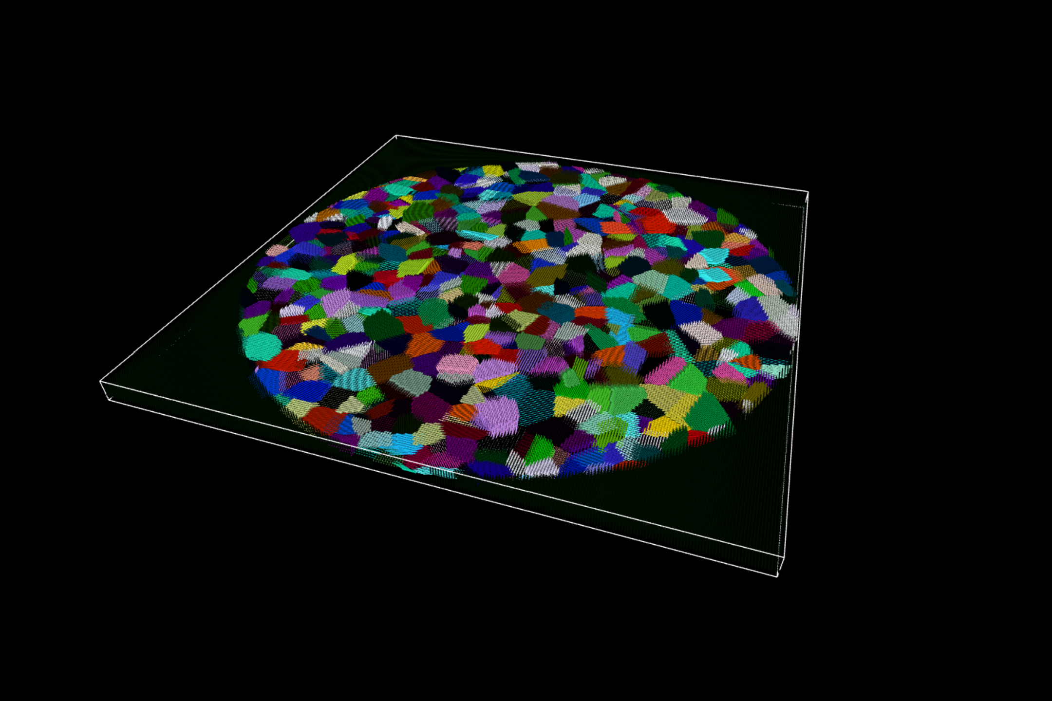
Magnetic geometry (300 nm x 100 nm x 3 nm) visualization in 3D using MuMax View in the browser:

---

More examples:

---

Related Animated Videos for Your Reference:
Tunnel Effect
Quantum Difference Between Metals & Insulators
Magnetic Orders
Frustrated Magnets
Bose-Einstein Condensation
Nuclear Magnetic Resonance (NMR)
Transmission Electron Microscopy
Scanning Tunneling Microscopy
Scanning Electron Microscopy
Atomic Force Microscopy

---

Additional helpful information

The specific magnetic topology determines the non-equilibrium dynamics governing collective excitations. A spin chain, defined as a one-dimensional sequence of exchange-coupled localized moments, is frequently modeled using one-dimensional Heisenberg or Ising Hamiltonians. Expanding this dimensionality yields a spin lattice, which is a periodic two- or three-dimensional crystalline arrangement supporting bulk magnonic wave propagation. These structures allow for the precise calculation of dispersion relations for localized excitations moving across the atomic array, thereby enabling the evaluation of long-range magnetic ordering and structural phase transitions.

Term	Core Characterization	Domain of Application	Mathematical Variable
Spin Cluster	A finite collection of strongly interacting localized magnetic moments.	Molecular magnetism, nanoscale devices.	$\hat{H}{cluster} = -\sum J{ij} \hat{\mathbf{S}}_i \cdot \hat{\mathbf{S}}j$, defining the exchange interaction $J{ij}$ between distinct spin vector operators $\hat{\mathbf{S}}_i$.
Spin Bath	An uncontrollable environmental continuum inducing decoherence upon a target qubit.	Open quantum systems, solid-state defects.	$\hat{H}_{SB} = \sum \mathbf{A}_k \cdot \hat{\mathbf{S}} \otimes \hat{\mathbf{I}}_k$, characterizing the coupling tensor $\mathbf{A}_k$ connecting the primary spin $\hat{\mathbf{S}}$ and nuclear bath spins $\hat{\mathbf{I}}_k$.
Spin Ensemble	A macroscopic collection of $N$ identical isolated magnetic moments addressed collectively to amplify signal strength.	Quantum memory, nuclear magnetic resonance.	$\hat{S}{\alpha} = \sum{i=1}^{N} \hat{\sigma}_{\alpha}^{(i)}$, characterizing the collective macroscopic spin operator along axis $\alpha$ for $N$ individual emitters.
Spin Chain	A one-dimensional sequence of exchange-coupled moments.	Low-dimensional magnetism.	$\hat{H}_{chain}$, representing the Hamiltonian dictating one-dimensional nearest-neighbor interactions.
Spin Lattice	A fully periodic multidimensional crystalline arrangement of interacting moments.	Condensed matter physics, spintronics.	$\hat{H}_{lattice}$, characterizing the bulk Hamiltonian governing global dispersion relations.
Spin Glass	A disordered collective state exhibiting geometric frustration and random exchange couplings.	Disordered magnetics, complex systems.	$\hat{H}{EA} = -\sum J{ij} \sigma_i \sigma_j$, representing the Edwards-Anderson model for localized Ising variables $\sigma_i$.
Spin Liquid	An extensively entangled macroscopic state possessing zero long-range magnetic order at absolute zero.	Topological quantum computing.	$\Psi_{QSL}$, representing the extensively entangled non-ordered ground state wavefunction.
Spin Texture	A spatially continuous, topologically protected field configuration of magnetic moments.	Nanomagnetism, skyrmionics.	$\mathbf{m}(\mathbf{r})$, representing the localized continuous magnetization vector mapping across spatial coordinates $\mathbf{r}$.
Spin Impurity	A solitary isolated magnetic moment embedded within a non-magnetic host matrix.	Quantum sensing.	$\hat{H}_{imp}$, detailing the localized zero-field splitting and Zeeman energy of a singular defect.

Finite spatial boundaries characterize a spin cluster as a discrete collection of strongly interacting localized moments typically synthesized within molecular magnets. Truncating the physical size alters the allowable energy eigenvalues, isolating discrete transition spectra completely distinct from bulk continuous bands. An extreme spatial reduction results in a spin impurity, constituting a solitary magnetic moment embedded within a crystalline host matrix. Solid-state physicists leverage these isolated defects, including nitrogen-vacancy centers in diamond, as single-spin quantum sensors or individual addressable qubits.

Macroscopic addressing of numerous identical emitters defines a spin ensemble. Simultaneous driving of these collective uncoupled spins by quantum hardware architects amplifies the resulting aggregate readout signal. Coupling such massive physical collections to microwave cavities provides superconducting circuits with robust quantum memories. The collective coupling strength scales asymptotically as $\propto \sqrt{N}$ relative to a solitary emitter. This scaling relation facilitates coherent information exchange operating well above the background thermal noise floor.

Uncontrollable environmental factors invariably disrupt coherent quantum operations. A spin bath constitutes a chaotic continuum of neighboring nuclear or electron spins interacting with a primary target qubit. This environmental distribution drives rapid decoherence by injecting randomized phase accumulations into the primary system. Mathematical modeling of this dissipative interaction requires characterizing the hyperfine coupling parameters defining the energy transfer between the central isolated spin and the surrounding stochastic field.

Disordered exchange couplings combined with geometric frustration generate complex collective phases lacking simple periodic alignment. A spin glass exhibits random ferromagnetic and antiferromagnetic interactions that freeze the localized moments into a disordered, metastable configuration. Conversely, a quantum spin liquid avoids freezing entirely, maintaining an extensively entangled, fluctuating macroscopic state possessing zero long-range magnetic order at zero kelvin. Topologically stable field configurations manifest as spin textures, mapping continuous spatial variations of the magnetization vector into protected formations resembling skyrmions or domain walls.

In summary, varying dimensionalities and interaction profiles dictate the specific terminology for magnetic collections. A spin chain or spin lattice describes ordered periodic arrays, a spin cluster represents a finite discrete molecular collection, and a spin bath identifies the chaotic environmental continuum driving decoherence. Driving $N$ identical non-interacting emitters simultaneously defines a spin ensemble, maximizing signal amplification for quantum memory applications. Complex disordered states include the frustrated spin glass, the extensively entangled spin liquid, and continuous spin textures. The absolute isolation of a single localized moment defines a spin impurity.

References

1. Bethe, H. (1931) ‘Zur Theorie der Metalle. I. Eigenwerte und Eigenfunktionen der linearen Atomkette’, Zeitschrift für Physik, 71, pp. 205–226. Supports: the one-dimensional Heisenberg spin chain, exchange interactions, and excitation eigenstates. https://doi.org/10.1007/BF01341708](https://doi.org/10.1007/BF01341708

2. Holstein, T. and Primakoff, H. (1940) ‘Field dependence of the intrinsic domain magnetization of a ferromagnet’, Physical Review, 58(12), pp. 1098–1113. Supports: spin-wave theory for interacting magnetic lattices and the mapping between spin operators and bosonic excitations. https://doi.org/10.1103/PhysRev.58.1098](https://doi.org/10.1103/PhysRev.58.1098

3. Gatteschi, D. and Sessoli, R. (2003) ‘Quantum tunneling of magnetization and related phenomena in molecular materials’, Angewandte Chemie International Edition, 42(3), pp. 268–297. Supports: finite exchange-coupled molecular spin clusters, quantum size effects, discrete magnetic energy levels, and magnetization tunneling. https://doi.org/10.1002/anie.200390099

4. Prokof’ev, N.V. and Stamp, P.C.E. (2000) ‘Theory of the spin bath’, Reports on Progress in Physics, 63(4), pp. 669–726. Supports: environmental nuclear and electronic spins, central-system coupling, and decoherence mechanisms; explicitly distinguishes localized spin baths from oscillator baths. https://doi.org/10.1088/0034-4885/63/4/204

5. Kubo, Y. et al. (2010) ‘Strong coupling of a spin ensemble to a superconducting resonator’, Physical Review Letters, 105(14), article 140502. Supports: collective coupling between a nitrogen-vacancy spin ensemble and a superconducting microwave resonator, demonstrated through vacuum Rabi splitting. https://doi.org/10.1103/PhysRevLett.105.140502

6. Edwards, S.F. and Anderson, P.W. (1975) ‘Theory of spin glasses’, Journal of Physics F: Metal Physics, 5(5), pp. 965–974. Supports: disordered magnetic interactions, competing exchange signs, frozen irregular spin configurations, and the theoretical foundation of the Edwards–Anderson description. https://doi.org/10.1088/0305-4608/5/5/017

7. Savary, L. and Balents, L. (2017) ‘Quantum spin liquids: a review’, Reports on Progress in Physics, 80(1), article 016502. Supports: quantum spin liquids as highly entangled phases without conventional magnetic long-range order, including fractionalized excitations, emergent gauge descriptions, and topological properties. https://doi.org/10.1088/0034-4885/80/1/016502

8. Fert, A., Reyren, N. and Cros, V. (2017) ‘Magnetic skyrmions: advances in physics and potential applications’, Nature Reviews Materials, 2, article 17031. Supports: skyrmions as topological magnetic textures, their stabilization through magnetic interactions, their dynamics, and proposed information storage and logic applications. https://doi.org/10.1038/natrevmats.2017.31

9. Doherty, M.W., Manson, N.B., Delaney, P., Jelezko, F., Wrachtrup, J. and Hollenberg, L.C.L. (2013) ‘The nitrogen-vacancy colour centre in diamond’, Physics Reports, 528(1), pp. 1–45. Supports: localized defect spins, nitrogen-vacancy electronic structure, zero-field splitting, magnetic interactions, and applications in quantum sensing and information processing. https://doi.org/10.1016/j.physrep.2013.02.001

10. Kubo, Y. et al. (2011) ‘Hybrid quantum circuit with a superconducting qubit coupled to a spin ensemble’, Physical Review Letters, 107(22), article 220501. Supports: experimental storage and retrieval of a superconducting qubit superposition through collective spin excitations, using a tunable superconducting resonator as the coupling bus. https://doi.org/10.1103/PhysRevLett.107.220501